While I’m taking Google’s Machine Learning Crash Course, I’ve got the idea of implementing a machine learning algorithm from scratch (but with a little help from NumPy for vectorization purposes). The first algorithm that I’ve implemented from scratch is Multivariate Regression. For this article’s example, I’ll be using a Linear Regression (a Multivariate Regression model with only one variable) example so that you can easily visualize the graphs.
I’ve used this dataset for this example. For graphs, I’ve used Matplotlib. I created a Python class named MultivariateRegression with these parameters on initialization:
- batch_size - The number of rows that will be used in computing the gradient. By default, all of the rows will be used in gradient computation.
- learning_rate - A scalar that will be multiplied to the gradient. By default, the value is 0.001.
- loss - Loss function that will be used, either l1 loss (absolute difference) or l2 loss (squared difference). By default, the squared difference will be used. You can read more about their differences here.
- num_epoch - The number of pass on the dataset. By default, the number of pass is 100.
Next would be the train function. First, we must add a bias column to the dataset. Think of it as the y-intercept of the line equation which can be generalized to . where is the number of weights/features and is the bias weight. This would result to a matrix where there are n rows and m columns (the number of features). In linear regression, we must find the best-fit line, which minimizes the error between the actual data and the predicted data (data point along the function line).
Mean Squared Error
The Mean Squared Error (MSE) will be the loss function which uses the squared differences to compute the error (the constant 2 from the denominator is for the derivative of the squared function so that they will cancel-out later).
To minimize this error, we must use the Gradient Descent algorithm.
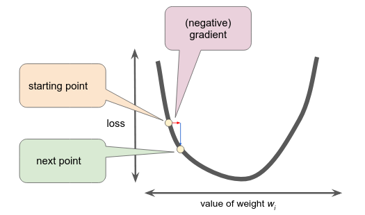
Gradient Descent
The main idea is, we have a bowl-like function graph which has the minimum value at the bottom and the goal is to reach the bottom. We can reach the bottom by computing the gradient of the function. The gradient is a vector of partial derivatives derivation of a function (I’ll leave the partial derivatives to you). The gradient vector will then be multiplied to the learning rate () and then the resulting value will be subtracted from the current weight value. Subtraction is performed since we are minimizing the error. Initially, the weights will be 0 (but you can choose any weights value if you want to experiment).
You can view the step-by-step computation of the gradient of the MSE here.
The new weights will then be computed using this formula:
After the number of epochs specified is reached, the training will then stop and the current weights will be used in future predictions. We will have a learned function of the form:
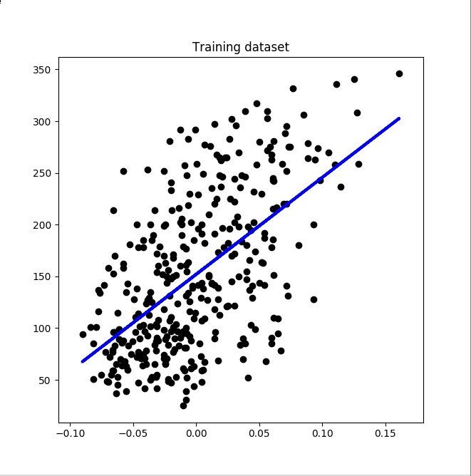
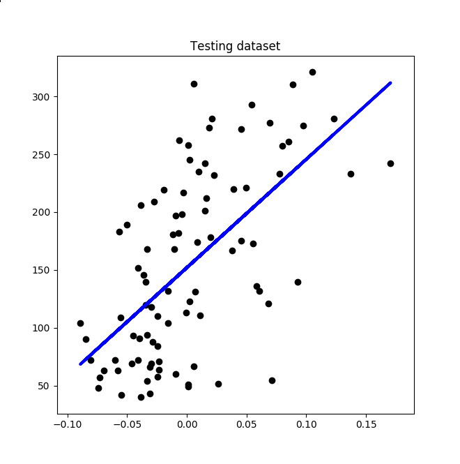
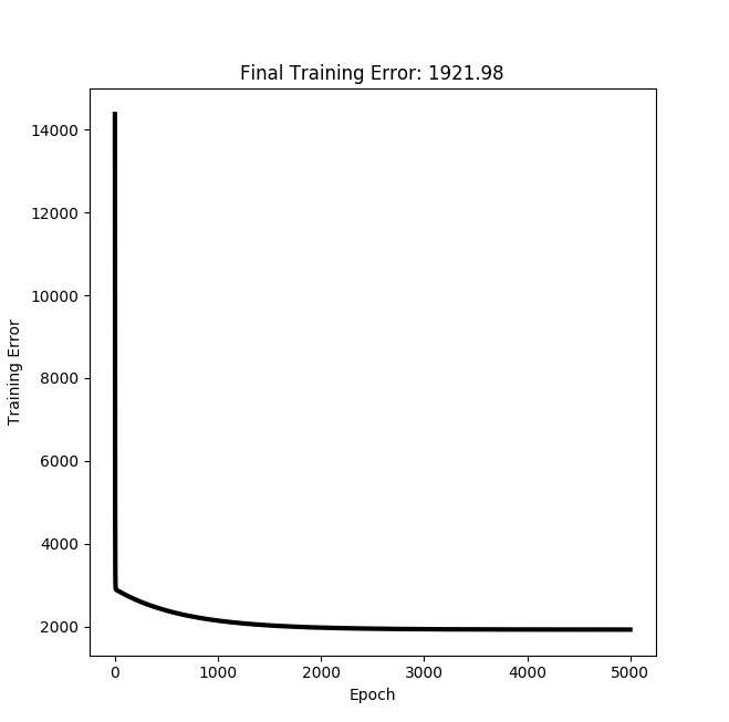
Results
Source Code
You can view the source code here: https://github.com/septa97/pure-ML/blob/master/pureML/supervised_learning/regression/multivariate_regression.py
Image references
Figure 1: https://developers.google.com/machine-learning/crash-course/reducing-loss/gradient-descent